Situational Awareness
Situation awareness with semantic region-landmarks
|
Permalink
Rupert Reiger, Anjan Sarkar, and Palash Goyal
19 November 2012
A semantic map-based localization and navigation method for unmanned aerial vehicles delivers encouraging results in simulations.
For autonomous systems, localization is a major precondition for situation-awareness—the observe, orient, decide, act (OODA) decision chain1, 2—and for navigation. The system has to first know where it is to build a picture of its environment and to gauge its placement relative to other surrounding objects. Then, the system can determine whether it is alone or in proximity with friendly or unfriendly others.
When an autonomous system localizes itself in an environment, it has to sense distinctive elements of its environment, so-called landmarks. Simultaneous localization and mapping (SLAM) uses landmarks to determine position in an environment and to simultaneously build a map of that environment. For example, imaging sensors—such as visible light and radar cameras ranges—can be used to perform SLAM. As reported by DeSouza and Kak a decade ago,3 autonomous system localization involves acquiring sensory information, detecting landmarks, matching observations and expectations, and calculating the autonomous systems' position.
The method of using particle filters, which is generally used to estimate a sequence of localization-relevant parameters, was first introduced by Murphy4 in 1999. In 2002, Montermerlo et al.5, 6 developed the FastSLAM algorithm, which uses particle filters rather than the extended Kalman filters used previously in SLAM. To summarize, Kalman filters represent probability distributions using a parameterized Gaussian model, whereby values with smaller estimated errors are ‘trusted’ more in formulating a probability bell curve of position. Particle filters instead represent location probabilities using a list of sample states called particles. Both methods are Bayesian in nature. The particle filter method has the benefit that it can encapsulate an estimate of an autonomous system's position alongside supplementary information, such as an extended Kalman filter (EKF) estimation of the position of landmarks.
FastSLAM 2.0, a further improvement to SLAM, was discussed by Montemerlo, Thrun, Koller, and Wegbreit.7 This systems makes a more-efficient use of the particle filter principle, particularly in situations where motion noise is high relative to measurement noise. FastSLAM 2.0 is also better than other algorithms at overcoming the data association problem, which can arise when different landmarks in the environment look alike. The classic solution to the data association problem in SLAM is to select a feature on the landscape such that it maximizes the likelihood of the sensor measurement given all available data, and to align all other data based on this step. FastSLAM 2.0 solves the problem by calculating the maximum likelihood for each particle, meaning that the additional step is not needed.
The basis of all SLAM variants can be thought of as a person localizing herself when navigating: looking around an urban environment, she recognizes landmarks such as buildings and streets. Considering elements of a journey (such as distance walked) helps build an internal sense of placement relative to surroundings—landmarks—for our navigator. Similarly, the question ‘how far have we travelled?’ is used in SLAM as the basis for localization alongside landmark detection. Another way people localize is to look at a scene in their field of view and go through a series of mental steps, such as: 'I see a lake; behind it I see a village; left of it is a forest; on the right there are fields—and before it I see grassland. It's clear, therefore, that I must be here, or if not here.' Moving through the landscape and subconsciously following the same mental steps eventually rules out possible alternatives, enabling the person to identify their location. Our implementation of SLAM works in the same way: as long as structures for landmarks can be found, SLAM enables a map to be built. Alternatively, when our human is in Antarctica in a white out, she can not localize, and neither can SLAM.
In our simulation, an unmanned aerial vehicle (UAV) attempts to keep to a pre-programmed route, taking pictures of the ground at regular intervals. The vehicle has only rudimentary land-cover information and has not previously mapped any region. The system analyses the images taken by the UAV and its control information. First, it splits up the map into areas described by semantic tags, such as urban, closed forest, open forest, deep water, shallow water, sand, and mineral-rich ground. It does this by referring to a look-up table, which contains optical and radar characteristics of different ground types that have been semantically tagged. After splitting the sensor images into different clusters of pixels, it computes the mean and variance optical characteristic of each cluster and tags them based on the values in the look-up table.
Using this method of semantic tagging, FastSLAM 2.0 provides a ‘best-estimated’ position, employing semantic neighbourhood tree structures called region adjacency graphs (RAGs). This defines the distinctive landmarks we use for SLAM. A disadvantage of FastSLAM 2.0 is that, if landmarks are sparse or measurement noise is high, the algorithm is prone to diverge. The essence of our approaches deals with these two drawbacks. Firstly, measurement noise is controlled by segmenting the images. Secondly, it defines landmarks with closed bounding regions.
We used a method described previously,8 using a Dempster-Shafer (DS) model for the best probabilistic fusion of visible light and radar data on a pixel level and classification, and Markov Random Fields (MRFs) for the segmentation for our land-cover model, all carried out while the UAV flies over a region. Dempster-Shafer is a mathematical theory of the believability of evidence, whereas MRFs are random variables that can be described by an undirected graph, whereby the edges represent dependencies, here neighbouring pixels' interactions for segmentation. Consequently, we call our model DS-MRF-RAG-FastSLAM.
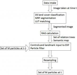
Figure 1 shows the workflow for the system we used. For the UAV's localization and navigation, we built a RAG that identifies a segment and neighbouring segments' land coverage, represented as a tree structure. The RAG's root, which describes the regions land cover, is fixed to the map's segments. The RAGs deliver distinctive landmarks that are unique enough to restrain the data association problem, especially in a limited region. Finally, FastSLAM 2.0 is used with the UAV's controls and the landmarks as input for simultaneous localization and mapping. To make the necessary comparison of the landmarks, a trees-comparing metric is used, measuring how well landmarks fit together. The metric delivers a parameter used to rank particles, with the best on top.
Figure 1.
Work flow for semantic map navigation using FastSLAM—fast simultaneous localization and mapping. DS: Dempster-Shafer. EKF: Extended Kalman filiter. LUT: Look-up table. MRF: Markov random fields. RAG: Region adjacency graph. t: Time.
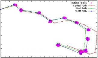
Figure 2 shows trajectories as calculated, with the real path and SLAM path correlating well. The concentration of the particles at different time steps suggest that the particles' positions can be corrected by the developments in new iterations of the SLAM software (which minimize the difference between expected observation and actual observation) to pull back the SLAM path onto the real path.
Figure 2.
An example of a trajectory of an unmanned aerial vehicle (UAV) as viewed from above.
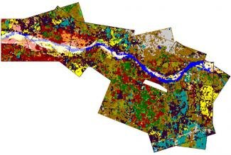
Figure 3 shows the semantic map with segments and land coverage coding (as colours) as generated by the UAV, set up by rectangles representing the regions seen by the camera at discrete time steps. The variable size of the rectangles correlates with the variable elevation over ground of the UAV. The RAGs attached to segments and building the landmarks are not shown.
Figure 3.
Map built online by the UAV flying the path in Figure 2.
In summary, our DS-MRF-RAG-FastSLAM approach is a powerful localization and navigation tool that is particularly suited to UAVs. It can also be fused with GPS- based methods, but shows the highest potential operating in situations in which GPS has been screened or jammed. In our simulation, we considered a 3D UAV position: two cartesian dimensions (x,y) and one rotational, the UAV's yaw. That is very reasonable because estimating altitude is difficult by looking down cameras at landmarks using SLAM. Thus, we estimated altitude as being a particular distance by measuring other sensor inputs. In the near future we hope to explore the possibility of including sensors roll, yaw and pitch angles to determine the volumetric environmental map. Using this type of system we would like to proceed to developing unguided UAVs capable of autonomous decision making.1
Authors
Rupert Reiger
EADS Innovation Works, EADS Deutschland GmbH
Anjan Sarkar
Department of Mathematics IIT Kharagpur
Palash Goyal
Department of Computer Science IIT Kharagpur
References
-
R. Reiger, Intelligent systems from the integrator company perspective, sound mathematical methods, World Congr. ICT Dev., 2009.
-
F. P. B. Osinga, Science, Strategy and War: The Strategic Theory of John Boyd, Routledge Chapman & Hall, 2006.
-
G. N. DeSouza and A. C. Kak, Vision for mobile robot navigation: a survey, IEEE Trans. Pattern Anal. Mach. Intell. 24 (2), pp. , 2002.
-
K. Murphy, Bayesian map learning in dynamic environment, Adv. Neural Inf. Process. Syst., pp. , 1999.
-
M. Montemerlo, S. Thrun, D. Koller and B. Wegbreit, FastSLAM: a factored solution to the simultaneous localization and mapping problem, Proc. AAAI Nat'l Conf. Artif. Intell., pp. , 2002.
-
M. Montemerlo and S. Thrun, Simultaneous localization and mapping with unknown data association using FastSLAM, IEEE Proc. Int. Conf. Rob. Autom. 2, pp. , 2003.
-
M. Montemerlo, S. Thrun, D. Koller and B. Wegbreit, FastSLAM: an improved particle filtering algorithm for simultaneous localization and mapping that probably converges, Proc. Int. Joint Conf. Artif. Intell., 2003.
-
A. Sarkar, A. Banerjee, N. Banerjee, S. Brahma, B. Kartikeyan, M. Chakraborty and K. L. Majumdar, Landcover classification in MRF context using Dempster-Shafer fusion for multisensor imagery, IEEE Trans. Image Process. 14 (5), pp. , 2005.
DOI: 10.2417/3201211.004383